Determine Putative Cells
The BD Rhapsody™ Sequence Analysis Pipeline provides the following options to determine putative cells:
- Basic Algorithm for mRNA, AbSeq, and ATAC-Seq
- Refined Algorithm for mRNA and AbSeq
- Refined Algorithm for ATAC-Seq
Ideally, the number of unique cell labels detected by the BD Rhapsody™ Sequence Analysis Pipeline should be similar to the number of cells captured and amplified by the BD Rhapsody™ workflow. However, various processes throughout the workflow can introduce noise that contributes to extra cell labels seen during sequencing analysis, including:
- Poor quality sample with ambient RNA present
- Hybridization of polyadenylated (polyA) oligonucleotides to non-cell beads residing in neighboring wells when the cell lysis step is too long
- Under-loading beads in BD Rhapsody™ cartridges, resulting in cells in a well without a bead, and thus the RNA from the cells diffusing to adjacent wells
- Low-level oligo contamination during bead synthesis
- Errors generated during the PCR amplification steps of the workflow
To distinguish cell labels associated with true putative cells from those associated with noise, the basic cell calling algorithm is used by default for all assays. When improved sensitivity or specificity of detecting putative cells is desired, refined algorithms are available for mRNA/AbSeq and ATAC-Seq.
For multiomics data (mRNA and ATAC-seq), different options are available for putative cell calling. Please check out Putative cell calling with multiomics data for details.
Basic algorithm for putative cell identification using second derivative analysis
The principle of the basic cell calling algorithm is that cell labels from actual cell capture events should have many more reads associated with them than noise cell labels. For mRNA/Abseq data, the basic algorithm is performed using read counts from mRNA molecules (by default) or from Abseq. All reads associated with RSEC adjusted molecules from the selected bioproduct type (mRNA by default) are taken into account. For ATAC-Seq, the basic algorithm is performed using the number of transposase sites in peaks.
Demonstrated in the figure below, the cumulative number of reads is plotted on a log10-transformed curve, with cells sorted by the number of reads in descending order (left image). Additionally, the rate of change of the cumulative count is calculated with the second derivative (right image). In a typical experiment, a distinct inflection point is observed in the second derivative, indicating a division between signal cell labels and noise cell labels (red vertical line). Cell labels to the left of the red vertical line are most likely derived from a cell capture event and are considered as signal. The remaining cell labels to the right of the red line are noise.
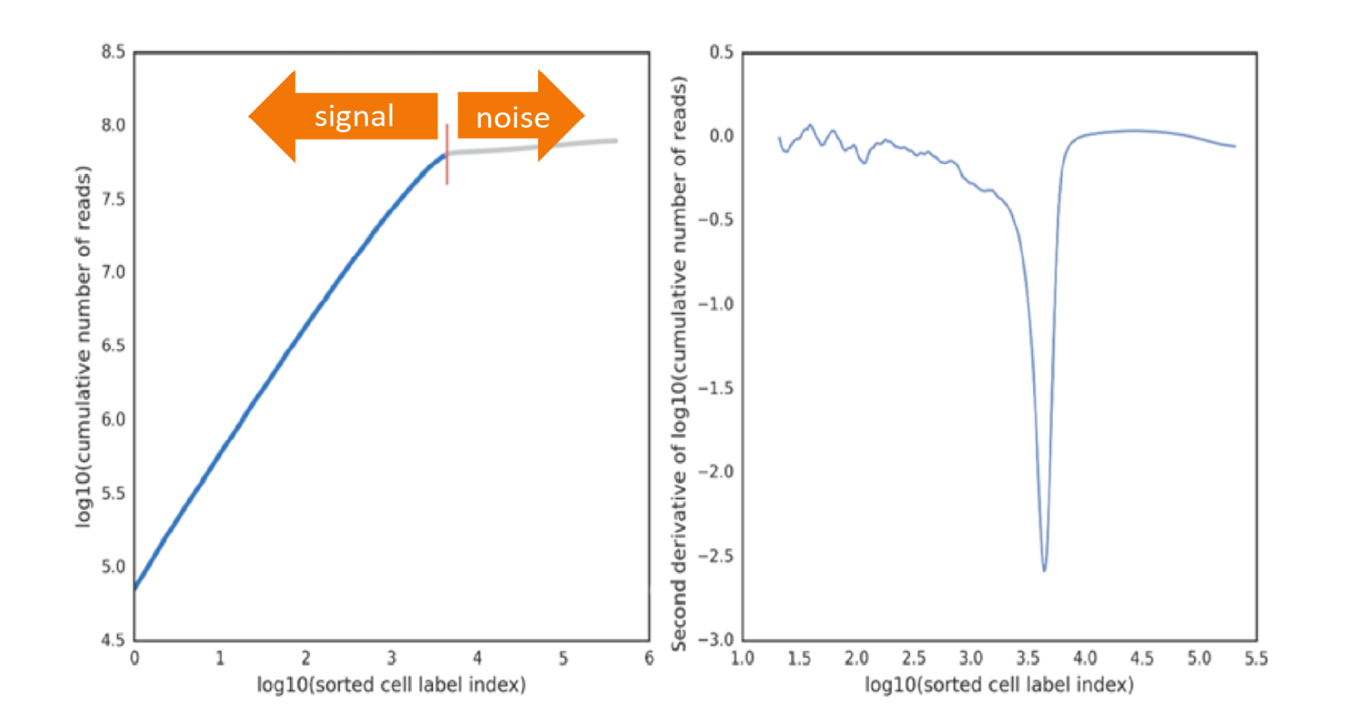
To find inflection points (minima in the second derivative curve), the algorithm first shifts the curve to be fully negative and determines the mean value along the full length of the curve. Then, local minima on the second derivative curve are progressively checked if they are at least 2.0x, 1.75x, or 1.5x deeper than the mean. At each multiple level, if at least one minima was found to surpass the depth, further multiples are skipped. If no minima surpass the 1.5x deeper than mean threshold, that is an indication that there is very little separation between signal and noise. In this case, the deepest minima is selected, but it suggests there may be a problem with the sample quality or cartridge protocol adherence.
If every cell in the sample is well represented by molecules from library preparation, there is only one inflection point. The number of reads of the putative cells is a single distribution well separated from the noise distribution.
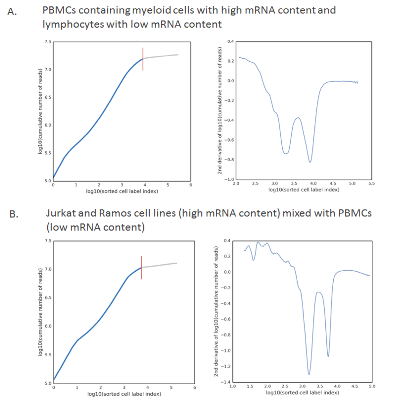
There are situations, however, when a sample contains cells with a very wide range of number of molecules. If major sub-populations of cells include those with high and low mRNA content, multiple inflection points can be observed. Example scenarios include biological samples like peripheral blood mononuclear cells (PBMCs) where myeloid cells often contain twice the mRNA content as lymphocytes (A. below), or artificial mixtures of cell line cells and primary cells (B. below). Targeted panels with an uneven representation of genes expressed in different cell types of a sample can also lead to multiple inflection points.
When multiple inflection points are found, there are several factors that go into choosing the cell call. The algorithm will pick the inflection point reflecting the highest number of cells which satisfy these criteria:
- Less than the dynamic maximum cell count. The dynamic maximum cell count is the greater of 1,000, or 60% of the number of total cell labels with read counts >= 10
- The read count per cell at the chosen inflection point is greater than 50 reads for all assays, except for
VDJcell calling, where the thresold is 75 reads per cell
These criteria are only applied in a multiple inflection point scenario. If there is only one inflection point deep enough, that cell call will be used.
The above multiple inflection point criteria can also be overridden by setting the Expected_Cell_Count pipeline
parameter. When set, the chosen inflection point will be the one closest to the provided Expected_Cell_Count. Although
this pipeline parameter is optional, it is good practice to provide it. Usually it can be set to the number
of cells loaded into the BD Rhapsody™ cartridge.
Refined algorithm for adjusting putative cell counts for mRNA and AbSeq
In some cases, the basic implementation of the second derivative analysis might include small numbers of false positive and false negative cell labels. If the refined algorithm is selected, additional refinement steps are run to attempt to identify these false positive and false negative cell labels.
Removing false positives
Consider the case where the chosen inflection point includes the populations of cell labels with wide ranges of number of reads per cell label. Then, the signal population with lower reads per cell label might also include noise cell labels derived from residual mRNA molecules from the cells with very high mRNA content. The number of reads associated with these noise cell labels derived from high-expressing cells can be indistinguishable from low-expressing cells, which have similar reads per cell.
Since these false positive cells can be hard to identify with reads alone, the relative expression profile of cell labels can be used to identify them. For example, a false positive cell label that is derived from a high mRNA-expressing, true positive cell label would likely have a similar expression profile but with a lower read signal. Therefore, a second derivative analysis is done on the most variable genes to identify these false positive cell labels.
The most variable gene expression is defined by a process similar to that described by Macosko, EZ, et al. (see References) :
-
Log-transform read counts of each gene within each cell to get the gene expression: log10 (count + 1).
-
Calculate the mean expression and dispersion (defined as variance/mean) for each gene.
-
Place genes into 20 bins based on their average expression.
-
Within each bin, calculate the mean and standard deviation of the dispersion measure of all genes, and then calculate the normalized dispersion measure of each gene using the following equation:
Normalized dispersion = (dispersion – mean)/(standard deviation) -
Apply a cutoff value for the normalized dispersion to identify genes for which expression values are highly variable even when compared to genes with similar average expression.
A second derivative analysis is applied on variable gene sets defined by a different cutoff value for the normalized dispersion to derive the cell label filtered set B. For each dispersion cutoff, the noise cell labels are determined as A–B. For instance, for three cutoff values, noise cell labels are N1 = A–B1, N2 = A–B2, and N3 = A–B3, where the minus sign represents the set difference. The common noise cell labels detected among N1, N2, and N3 are subtracted from cell labels set A (those identified by the basic algorithm). The resultant set is denoted as cell label filtered set C = A – intersection(N1, N2, N3).
Recovering false negatives
Cells with low numbers of molecules might be missed by the basic implementation of the second derivative analysis algorithm, because a cell subset might express very few of the genes in the (Targeted assay) gene list. The cell labels carry a very low number of reads, and the size of the cell population is small enough that their cell labels do not form a distinct second inflection point. These cell labels might be mistaken as noise.
If there are genes specific to the false negative cell label subset (for example, marker genes), they can be identified by comparing the number of reads for each gene from all detected cell labels to those from cell labels deemed as signal. The assumption is that the relative abundance of reads for each gene from all of the noise cell labels should be no different than that from all of the cell labels considered as signal. If a specific cell subset is missed initially, there is a set of genes that appears as enriched in the noise cell labels in the basic implementation.
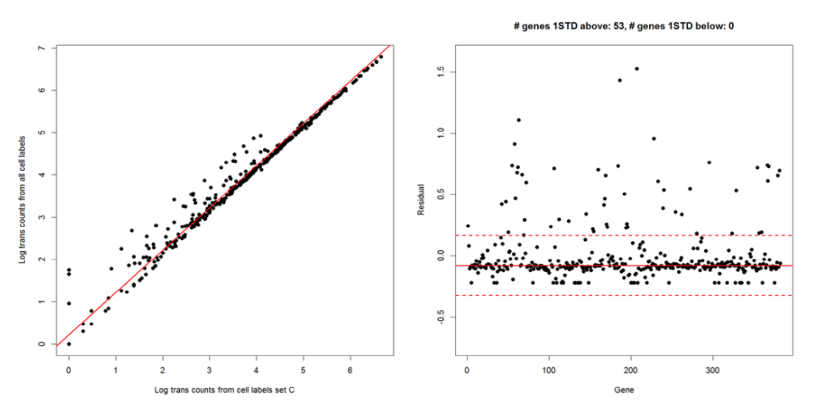
Left and right images below: Detecting genes enriched in noise as determined by the basic implementation of the second derivative analysis. Each dot represents a gene. This enriched set of genes is detected by the following steps:
- For each gene, calculate the total read counts from all detected cell labels and from cell labels in set C.
- Identify the genes that have the biggest discrepancy in representation by cell labels in set C versus all cell labels. This is done by plotting and finding the line of best fit to detect the genes with the largest residuals at least one standard deviation away from the median of residuals of all genes.
The two red dashed lines correspond to one standard deviation above and below the median (red solid line). In this
example, 53 genes are enriched in the noise population.
The second derivative analysis algorithm is run again with this enriched set of genes. The recovered cell labels (cell label filtered set D) are combined with cell labels in set C to form set E. As a final cleanup step, cell labels carrying less than the dynamically determined minimum threshold number of molecules are removed. The number of cell labels in the final set is the number of putative cells from the refined algorithm.
Refined algorithm for adjusting putative cell counts for ATAC-Seq
In some cases, the basic implementation of the second derivative analysis might include small numbers of false positive and false negative cell labels. If the data quality is not ideal, it may be difficult to separate the signal from the noise using only the number of transposase sites in peaks. If the ATAC-Seq refined algorithm is selected, a Guassian Mixture Model (GMM) approach is used to determine putative cells using two metrics: the number of transposase sites in peaks and the fraction of transposase sites in peaks.
The ATAC-Seq refined algorithm has five main steps:
- Filter out low-quality cell labels using the fraction of transposase sites in peaks
- Filter out low-quality cell labels using the number of transposase sites in peaks
- Identify a putative cell cluster using the number of transposase sites in peaks - the first GMM
- Identify a putative cell cluster using the number of transposase sites in peaks and fraction of transposase sites in peaks - the second GMM
- Refine the boundary of the putative cell cluster
The first two steps filter out low-quality cells, the third step identifies a putative cell cluster using the number of transposase sites in peaks (the first GMM), the fourth step identifies a putative cell cluster using both the number of transposase sites in peaks and the fraction of transposase sites in peaks (the second GMM), and the last step refines the boundary of the putative cell cluster. The first two steps filter out low-quality cell labels using the fraction of transposase sites in peaks and the number of transposase sites in peaks, respectively. The filtering in steps 1 and 2 improve the fit of the first and second GMMs in steps 3 and 4 where the boundary of the putative cell cluster is determined. The last step further refines the boundary of the putative cell cluster, either by recovering false negative cell labels or by filtering out false positive cell labels.
Filter out low-quality cell labels using the fraction of transposase sites in peaks
The cell labels with a low fraction of transposase sites in peaks show low specificity in targeting open chromatin sites. Those cell labels might have been generated due to several reasons such as inefficient transposase activity or non-ideal cell conditions. The threshold for the fraction of transposase sites in peaks is 0.1. Any cell labels with a fraction of transposase sites in peaks below 0.1 are filtered out.
Filter out low-quality cell labels using the number of transposase sites in peaks
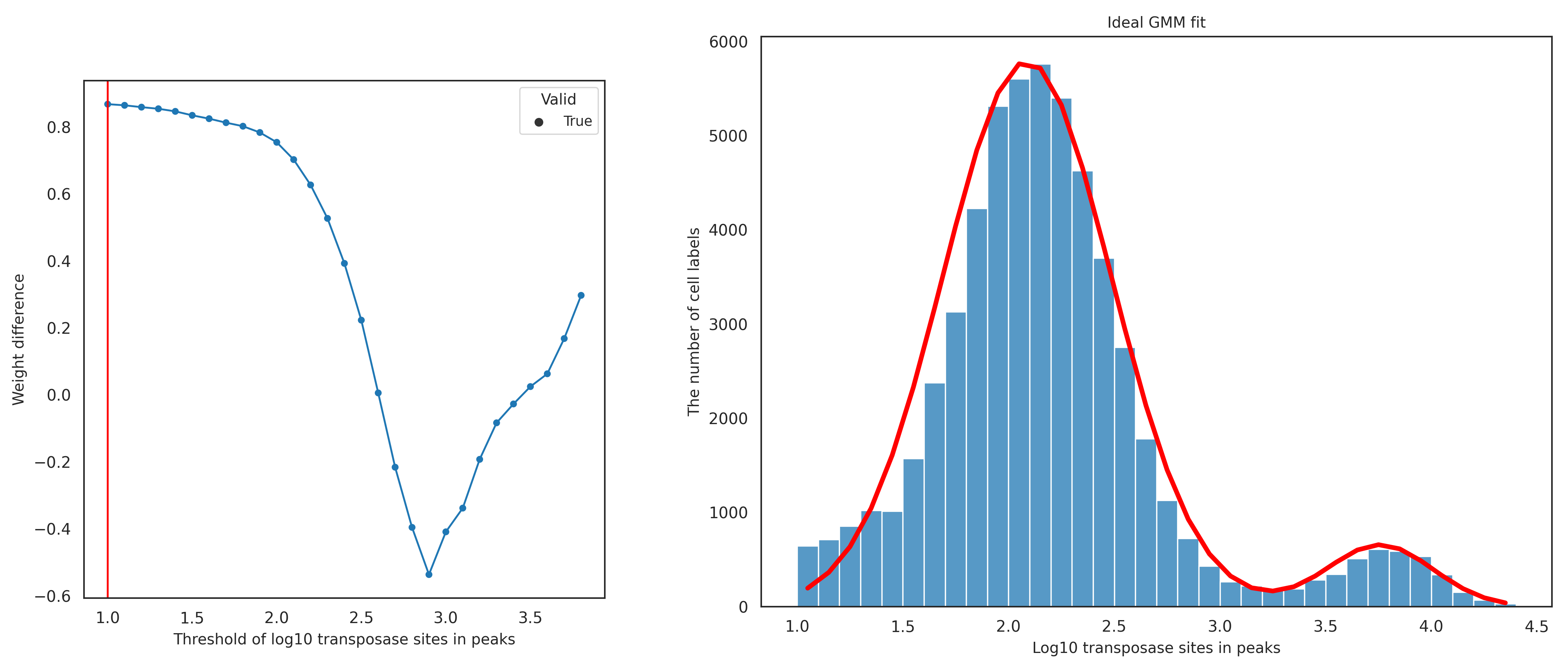
The cell labels with a low number of transposase sites in peaks show low sensitivity in the assay. The threshold for the minimum number of transposase sites in peaks is dynamically selected for each dataset as follows. The bottom and top 1% of the log10-transformed number of transposase sites in peaks are calculated and used as the lower and upper bounds of the dynamic threshold testing range. If the lower bound value is less than 1, meaning less than 10 transposase sites in peaks, the lower bound is set to 1. This adjustment is to avoid selecting an extremely small value for the threshold and to ensure that cell labels with low sensitivity are filtered out. Each possible threshold from the lower bound to the upper bound at a 0.1 interval is tested using the GMM approach. For each tested threshold, the cell labels having transposase sites in peaks below the threshold are filtered out, and the remaining cell labels are fitted into two clusters using the GMM approach. The difference of the GMM weights of the two clusters is calculated by subtracting the weight of the putative cell cluster (the cluster with a higher 90% confidence interval) from the weight of the non-cell cluster. If the 90% confidence intervals of the two clusters completely overlap, the tested threshold is considered invalid and is not selected for the final number of transposase sites in peaks threshold. After weight differences of all tested threshold are calculated, a stability score is calculated for each tested threshold by counting the number of times the weight difference value decreases in a row after that threshold.
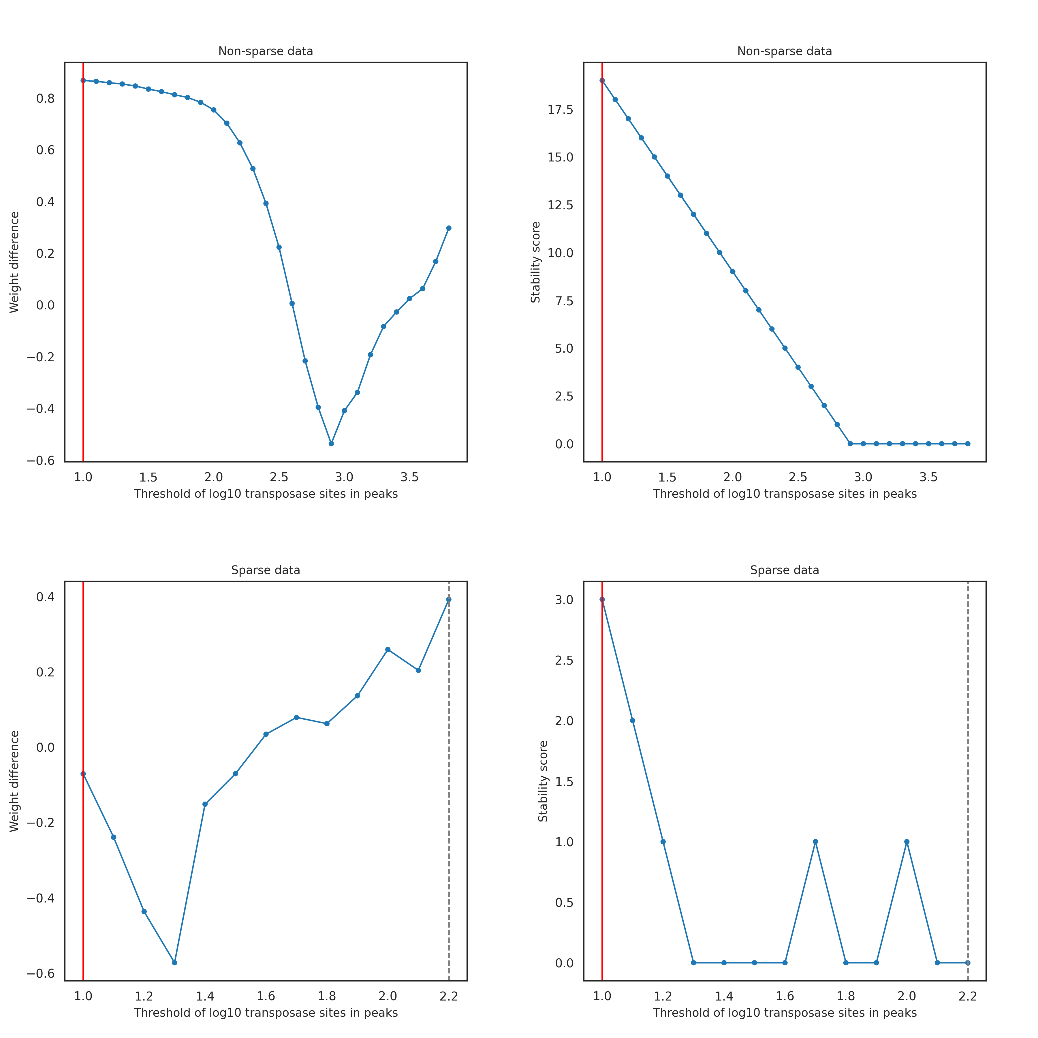
For good-quality data (left figure below), the weight difference usually decreases as the tested threshold value increases, because more cell labels from the non-cell cluster are filtered out. Then, the weight difference starts to increase when the majority of non-cell labels are filtered out and therefore the GMM starts to detect two sub-clusters within the putative cell cluster. This trend results in the tested threshold with the highest weight difference having the highest stability score. The figures below show an ideal GMM fit (right figure) when low-quality cells are properly filtered out using the final number of transposase sites in peaks threshold determined (left figure, red vertical line).
However, low-quality data with lots of noisy cell labels shows a different trend: as the tested threshold value of the number of transposase sites in peaks increases, the weight difference initially increases and then later follows the trend of good-quality data (left figure below). That initial increase is due to the abundance of noisy cell labels which causes the GMM to miss the putative cell cluster and instead identify two clusters in the non-cell labels, as shown in the right figure below. However, after the majority of non-cell labels are filtered out, the GMM starts to detect a putative cell cluster, causing the weight difference to plateau and then decrease. When the majority of non-cell labels are filtered out, the weight difference increases, similar to the good-quality data shown above. In this case, as shown for the good-quality data above, the tested threshold with the highest weight difference has the highest stability score.

In most cases, the tested threshold with the highest weight difference has the highest stability score (first row of figures below; the red line for the final threshold using the stability score). However, if data is too sparse, then the tested threshold with the highest weight difference may not have the highest stability score. With sparse data, the weight difference of a non-cell cluster and a cell cluster in an ideal GMM fit is not as significant as with non-sparse data. Thus, using the weight difference alone does not provide a stable measure of detecting a whole non-cell cluster. In this case, using the stability score results in a more robust selection of the threshold of transposase sites in peaks (second row of figures below; the red line for the final threshold using the stability score and the gray dotted line for the threshold chosen using weight difference).
With the reasoning above, among the valid thresholds, the threshold with the highest stability score is selected for the threshold of the number of transposase sites in peaks (red vertical line in images above) and used to filter out the low-quality cell labels. If there are multiple tested thresholds with the same stability score, the threshold with the highest weight difference is chosen. The rationale is that a high stability score of a tested threshold means the weight of the non-cell label cluster decreases sequentially as the threshold value increases, and that suggests a reliable removal of non-cell labels when higher thresholds are tested. That means the threshold with the highest stability score reliably detects the non-cell label cluster as a whole. Keeping a whole non-cell label cluster (excluding low-quality cells) is ideal. Losing many non-cell labels could lead to undesirable GMM fitting in the downstream steps where both clusters could be fit to the putative cell cluster rather than fitting one cluster to the putative cell cluster and the other to the non-cell clusters. The non-ideal GMM fit could result in false negative cell labels that are missed. The weight difference is also a rough estimate that shows when both a non-cell cluster and a putative cell cluster are detectable without losing many non-cell labels. If the weight difference is small, many non-cell labels may be filtered out. If the weight difference is large, then the low-quality cell labels are filtered out while preserving many non-cell labels, leading to the desirable GMM fit in the downstream steps. When there are multiple tested thresholds with the same highest stability score and the same largest weight difference, the largest threshold is chosen.
Identify a putative cell cluster using the number of transposase sites in peaks - the first GMM
After filtering out low-quality cell labels, the first GMM is performed on all remaining cell labels using the number of transposase sites in peaks. Two clusters are identified (a putative cell cluster and a non-cell cluster), and a cluster assignment is determined for each cell label. When the putative cell cluster and the non-cell cluster do not have good separation, the cell labels at the lower end of the number of transposase sites in peaks are sometimes assigned to the putative cell cluster. This happens due to a high variance estimated for the putative cell cluster. To better define a putative cell cluster using the number of transposase sites in peaks, the maximum value of the number of transposase sites in peaks from the non-cell cluster is calculated and used as the threshold to identify the putative cell cluster. The cell labels in the putative cell cluster proceed to the next step, the second GMM.
Identify a putative cell cluster using the number of transposase sites in peaks and fraction of transposase sites in peaks - the second GMM
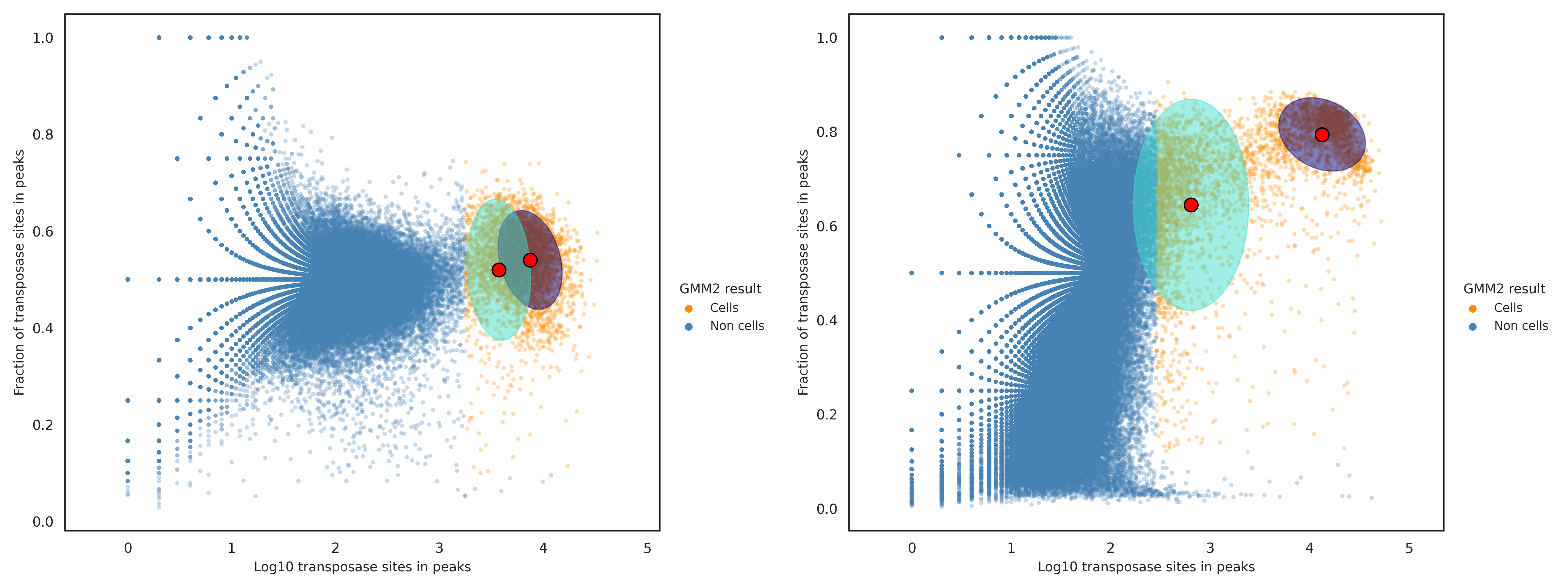
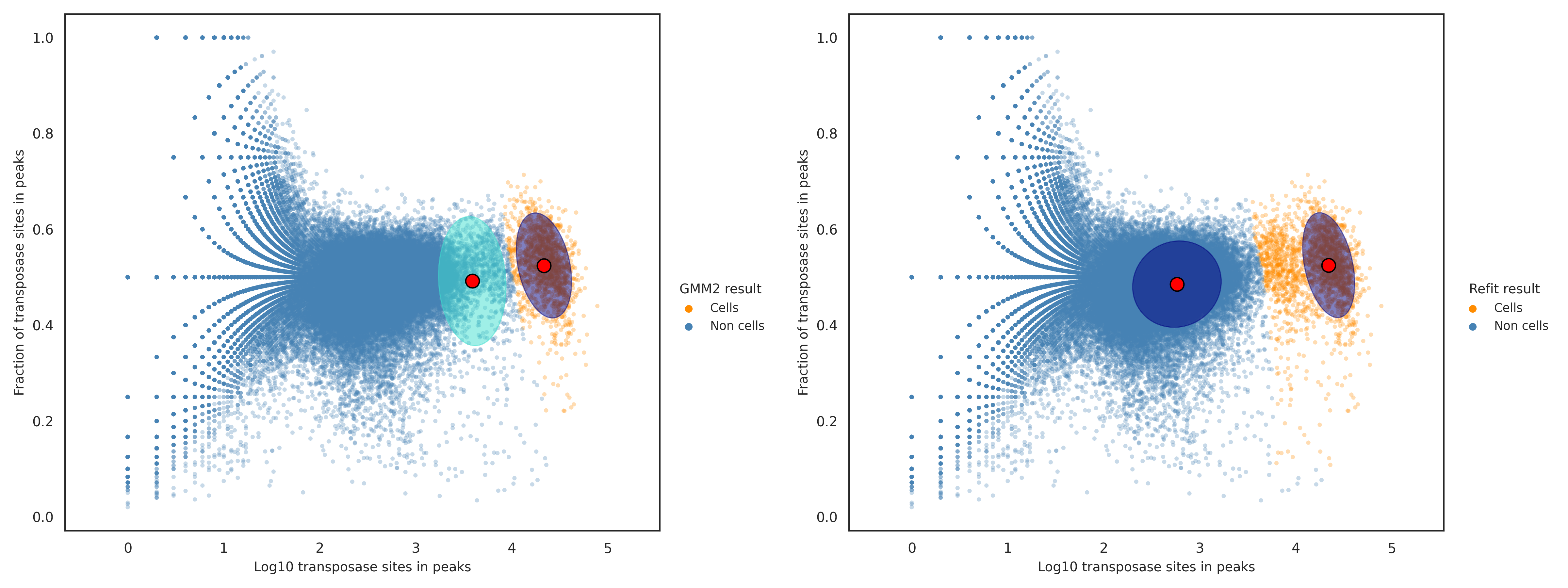
The cell labels in the putative cell cluster from the first GMM are evaluated using the second GMM, using both the number of transposase sites in peaks and fraction of transposase sites in peaks. The goal of the second GMM is to better define the boundary of the putative cell cluster in the two-dimensional space. The 90% confidence intervals (ellipses) of the two GMM clusters are determined and checked if they overlap. If the two confidence intervals overlap (left figure below), that indicates a lack of evidence that two distinct clusters exist and thus the second GMM result is ignored. In contrast, when the two intervals do not overlap (right figure below), that suggests that two distinct clusters exist and the boundary of the putative cell cluster is redefined; the cluster with a higher mean value for the number of transposase sites in peaks is considered a redefined putative cell cluster, and the cell labels assigned to that redefined putative cell cluster are identified as putative cells.
Refine the boundary of the putative cell cluster
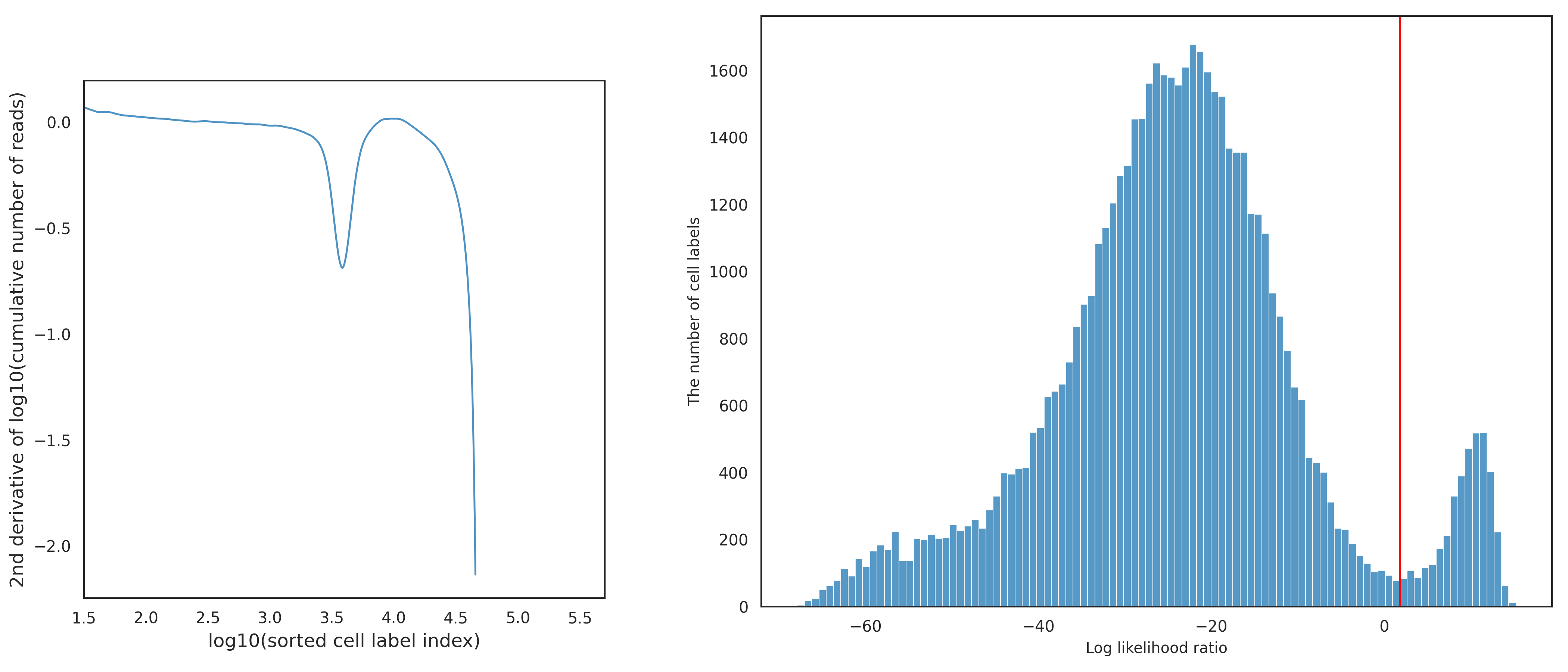
This final refitting step is aimed at improving the boundary identification of the putative cell cluster, either by removing false positives or recovering false negatives. If the previous second GMM result is ignored, the putative cell calling results could contain a small amount of false positives. If the previous second GMM result is applied, the putative cell calling results could be missing a small amount of false negatives. To further refine the boundary of the putative cell cluster in the two-dimensional space, the non-cell labels and the putative cell labels are fitted into two separate two-dimensional Gaussian distributions. Here, the non-cell labels are the cell labels filtered out from the first and second GMM, not including low-quality cell labels. Using the two resulting Gaussian distributions, a log likelihood ratio of the Gaussian distribution from the putative cell labels to the Gaussian distribution from the non-cell labels is calculated for each cell label. The threshold of the log likelihood ratio is dynamically determined for each dataset using the Basic Cell Calling Algorithm, but instead of using reads or transposase sites in peaks, the log likelihood ratios are used. Also, here, the half depth criteria is not used to select the inflection point. The figure below shows the second derivative curve (left) and the histogram of log likelihood ratios (right) with the red line being the selected threshold from the basic algorithm.
When the result from the second GMM in the previous step is ignored, the cell calling results could contain a small amount of false positive cell labels. The false positive cell labels are defined as cell labels having a log likelihood ratio less than the dynamically determined threshold from above, and are filtered out in this step. The figure below shows the putative cell and non-cell clusters before the false positives are removed (left) and after (right).
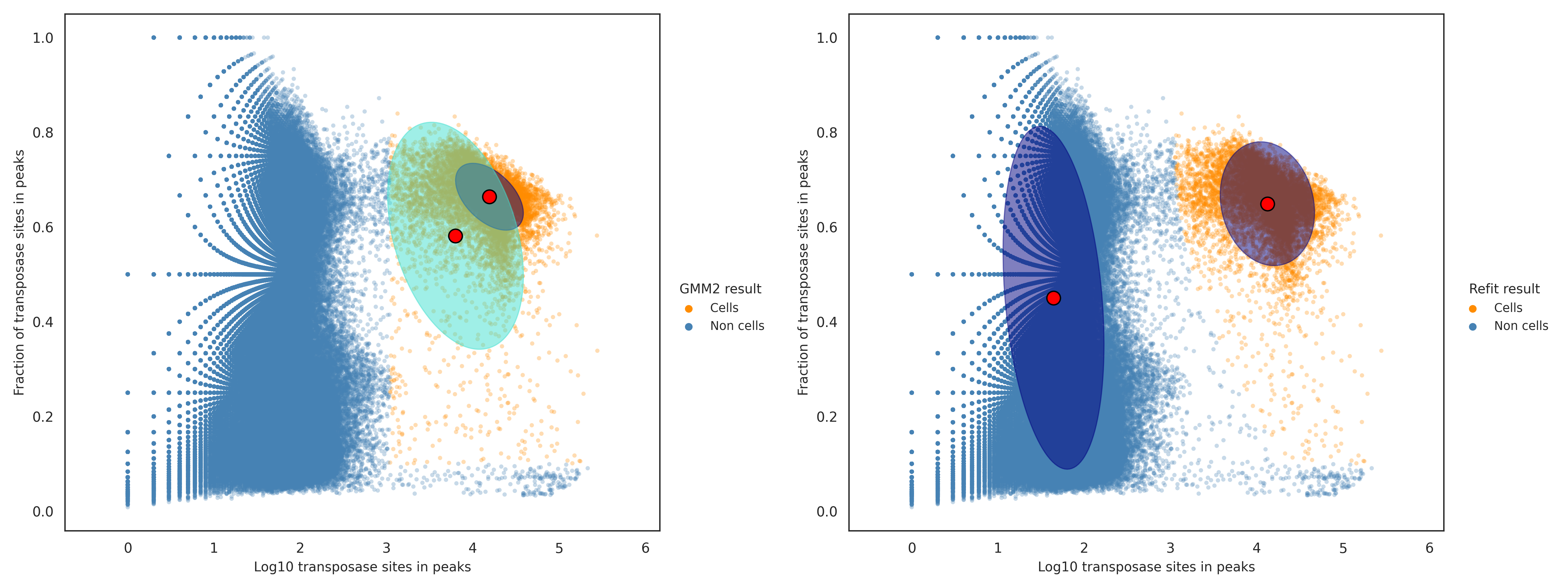
In contrast, when the result from the second GMM in the previous step is used to filter out non-cell labels, the cell calling results could be missing a small amout of false negative cell labels. The false negative cell labels are defined as cell labels having a log likelihood ratio greater than or equal to the dynamically determined threshold from above, and are recovered in this step. The figure below shows the putative cell and non-cell clusters before the false negatives are recovered (left) and after (right).
This step improves the robustness of the putative cell calling result, especially when the result from the second GMM in the previous step had a minimal overlap or a minimal gap between the two confidence intervals. This improved robustness comes from the log odds ratio threshold being dynamically chosen. If there was a minimal overlap in the confidence intervals from the second GMM, then the second GMM result was ignored, and the log likelihood ratio threshold chosen here would remove false positive cell labels. If there was a minimal gap between the two confidence intervals from the second GMM, then the second GMM result was used to filter out non-cell labels, and the log likelihood ratio threshold chosen here would recover false negative cell labels.
Identify Protein Aggregates from AbSeq Read Counts
When identifying putative cells using the AbSeq read counts, the basic implementation may include a small number of
false positive cell labels due to protein aggregates. Putative cells identified with high expression across most AbSeq
targets are considered protein aggregates. The protein aggregate status for each putative cell can be found in the
<sample_name>_Protein_Aggregates_Experimental.csv file. The cell label is marked True if it is considered a potential
protein aggregate and False if not.
Specifying an Exact Cell Count
If the user specifies a desired Exact_Cell_Count parameter with a value N, the cell labels are sorted by highest read
count (mRNA) or transposase-site-in-peaks count (ATAC), and the top N cell labels will be selected as putative cells
based on their ranking. If the Cell_Calling_Data parameter is set to mRNA_and_ATAC (requesting joint cell calling
in a multiomic experiment) and an Exact_Cell_Count parameter is specified,
the cells are sorted within each modality independently. The cells are then ranked by their
position among each modality, and the top N putative cells will be selected based on their average ranking across modalities.
Putative cell calling with multiomics data
With multiomics data (mRNA and ATAC-seq), the default putative cell calling option is joint cell calling by intersecting two putative cell lists derived from mRNA and ATAC-seq data. Alternatively, putative cell calling can be performed using only one of these assays. This approach might be useful in certain cases, for example, when data quality is optimal for only one assay. In such cases, putative cells will be initially identified using only the selected assay, and then the cells that do not exist in the unselected assay are filtered out. If a high percentage of putative cells are filtered out after initial identification, it could indicate suboptimal data quality. If an unusually high percentage of putative cells are filtered out, check if all the input sequencing libraries (Reads and ATAC_Reads) came from the same cells. If this is a run with SMK reads in the "Reads" input, ATAC reads in the "ATAC_Reads" input, and no mRNA reads (SMK and ATAC_Reads only), choose "Single-Cell Multiplex Kit - Nuclei - ATAC-Only" as the Sample Tag Version.